| |
Everything You Ever Wanted To Know About
Application Software:
Microsoft Excel
A
spread sheet is a piece of paper with rows and columns for recording financial
data for use in comparative analysis. In computer science, it is an accounting or
bookkeeping program that displays data in rows and columns on a screen. (Bartleby.com)
Even
though simple accounting procedures can be done using spreadsheets, there are
specific accounting packages which include different modules, such as accounts
receivable or accounts payable. Microsoft
Money and Intuit Quicken are two
accounting packages designed for home use.
The
main spreadsheet programs are Microsoft Excel, Lotus
1-2-3, and Quattro Pro. These
are several screen shots that will assist you in
creating a spreadsheet using Microsoft Excel. Some of the screens are actual links ... click on
them to see a full screen, which will make it easier to read! It will open
up in a new window, so when you want to return to this page, just "X"
out or close that browser window.
To
open Microsoft Excel, click on "Start"
~ "Programs"
~ "Microsoft
Excel."
Click on image to
enlarge
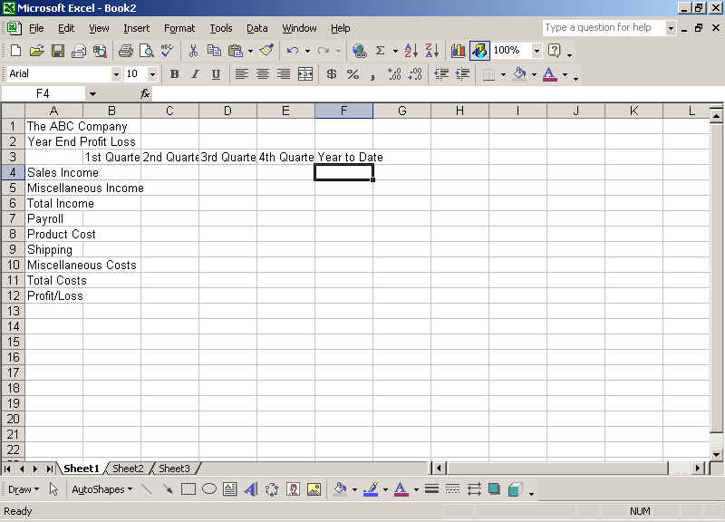
This is the first
screen that you will see. You should have some idea of what columns and
rows you will need to report all the information you want. However, you
can easily change the order of columns or rows using the cut and paste function
common to all Microsoft products.
A cell (or an area in
which data is keyed) is identified by the column and the row. For
instance, the first square in the top left hand corner is labeled
"A1," which is column A, row 1. Note that the toolbar across the
top of the screen is very similar to other Microsoft products, particularly in
the Microsoft Office package. Therefore, centering information, selecting
font styles and sizes, bolding, italicizing, and underlining is done in the same
way as in Word.
Click on image to
enlarge
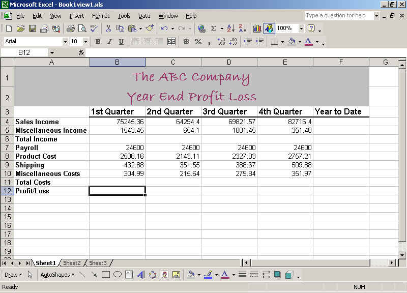
In cell A1, we entered
"The ABC Company" and in cell A2, we
entered "Year End Profit/Loss." In
cells, B3 through E3, we entered the 1st quarter, 2nd Quarter, 3rd Quarter, and
4th Quarter. In cell F3, we
entered "Year to Date." In cells A4
through A11, we entered sales income, miscellaneous income, total income,
payroll, product cost, shipping, miscellaneous costs, total costs, and in cell
A12 we entered profit/loss. To complete the rest of the spreadsheet
formatting, we did:
-
In Cells A1 and
B1,
selected Bradley Hand ITC font and selected 20
for the font size. Bold each cell.
-
Selected "plum"
for the font color and "gray-25%" for
the fill in the background (located to the left of the font color icon) for
both cells.
-
With cursor in
cell A1, we dragged the cursor to the right side of cell F1. With this
range highlighted, we clicked the merge and center
button, which is to the right of the left, center, right justifying
icons. Repeat for cell B1.
-
Highlight cells B3
through F3, Arial, size 12, bold.
-
Highlight cells A4
through A12, bold (Ariel, size 10).
-
On the gray
alphabetical bar on the top of the work sheet, place the cursor between
block "A" and block "B." The cursor changes to
crosshairs. Enlarge column A to 20.43 (or 148 pixels) by clicking and
dragging cursor to the left.
-
Increase columns B
through F to 15.00 (or 110 pixels).
-
Highlight B3 to
F3, and click on the borders icon to the very right of the fill color icon (two
from the font color icon). Select row 2 column 2, thick bottom border.
-
We keyed in the
following data, but it really doesn't matter what you key in as long as
there is data in the proper fields.
| |
1st Quarter |
2nd Quarter |
3rd Quarter |
4th Quarter |
| |
Column B |
Column C |
Column D |
Column E |
| Sales Income |
75245.36 |
64294.40 |
69821.57 |
82716.40 |
| Misc. Income |
1543.45 |
654.10 |
1001.45 |
351.48 |
| Payroll |
24600 |
24600 |
24600 |
24600 |
| Product Costs |
2508.16 |
2143.11 |
2327.03 |
2757.21 |
| Shipping |
432.88 |
351.55 |
388.67 |
509.88 |
| Misc. Costs |
304.99 |
215.64 |
279.84 |
351.97 |
Your worksheet should
now look like this:
Click on image to
enlarge
-
Highlight cells B5
through E5. Click the borders icon and add a bottom
border (row 1, column 2).
-
Highlight cells B6
through E6. Click on the "Auto Sum"
button which looks like the Greek letter, sigma ( )
on the tool bar above the comma (,). As you enter, you will see that
the total income for all 4 quarters is now shown. )
on the tool bar above the comma (,). As you enter, you will see that
the total income for all 4 quarters is now shown.
-
Highlight the
cells B10 through E10 and insert a bottom
border (row 1, column 2).
-
Follow the same
procedure as above for totaling cells B11 through E11.
Highlight, Auto Sum (),
enter.
-
Place cursor in
cell B12. Type the equal sign (=).
Point and click B6. Type the dash, or minus sign (-). Point and
click B11. Enter. Now you have the difference between total
income and total costs, or the profit-loss for
the quarter.
-
Click onto cell
B12, control C. Highlight C12 through E12, control V. The same
formula that was entered originally into B12 is now copied to row 12 of
columns C, D, and E. (Excel automatically updates the formula with the
proper cells.)
-
Highlight columns
F4 through F12, and use the "Auto Sum" ()
button to enter Year to Date totals.
-
Highlight cells B3
through F5. Right click, format cells.
(Or use the Format on the top toolbar.) On the Number tab, click
"number" and be sure that the 1000 separator (comma) is checked
and the decimal point is set at 2. Select the negative number format
of your choice. We chose the third one from the top, using brackets
and in black rather than red. Click OK.
-
Use the same
formatting steps as above to format cells B7 to F10.
-
Highlight B6
through F6. Right click, format cells. On the number tab, select
"accounting." The decimal place should be set at 2.
Click OK.
-
Follow the same
for B11 to F12 to format those cells.
-
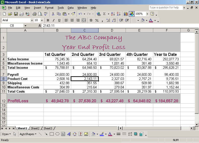
In the same way as
we lengthen the width of the columns, with the cursor as crosshairs, we
increased the height of row 7 by placing the cursor between the 7 bar and
the 8 bar to increase the height to 21.00 (or 28 pixels). We increased
row 12 to 30.00 (or 40 pixels) in the same way. (This gives the
spreadsheet more ease in reading.)
-
We also increased
the font in row 12 to size 12. Highlighting A12 through F12, we filled
with "gray-25%" and changed the font
color "plum." We also made this
range bold for ease in reading.
Click on image to
enlarge
Before you
print, you want to go to File, Page Setup, and change the orientation
from portrait to landscape in order to get the entire spreadsheet on one
8-1/2 by 11 sheet of paper.
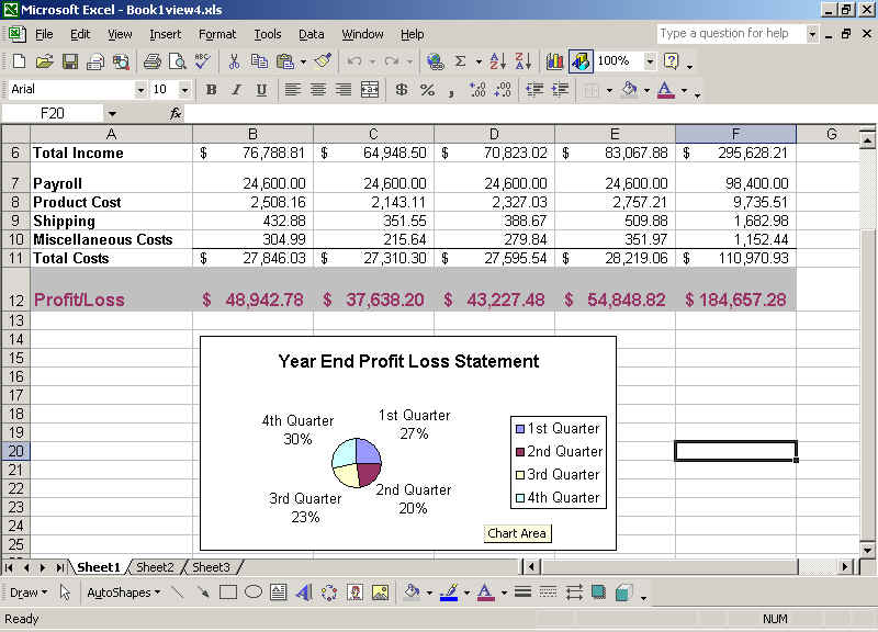
To create a simple
graph, highlight cells B3 through E3.
Holding down the control key, highlight cells B12 through E12. Click
onto the chart wizard - 3 icons to the right of the sigma icon ().
-
We selected
the pie graph and clicked next.
-
After
confirming that there was a check in "rows,",
we clicked on "next."
-
On the title
tab, we inserted the title of "Year End
Profit Loss."
-
On the legend
tab, we chose the legend to display on the right hand side.
-
On the data
labels tab, we chose "category,"
"percentage," and made sure that "show leader lines"
was checked.
-
We chose the
graph to be an object in the spreadsheet rather than creating a new
sheet for the graph. (This would of course depend upon how much
information is contained on the spreadsheet.)
-
Click finish.
Click on image to
enlarge
Microsoft
Access
Microsoft Excel
Microsoft Word
System Software
Return
to Main Page
Created by Brad Eaton and
Chris Sidebottom
Students at Hobart Middle
School, Hobart, Indiana
To report problems with this page or broken links, contact Webmaster
Copyright © 2003. All Rights Reserved
|