Pappos' Theorem

Pappos' Theorem is one of the most fundamental theorems in projective geometry. In a certain sense it is the smallest example of an incidence theorem. In this step-by-step example we will construct a draggable instance of the theorem.

Drawing Your First Point

When you start Cinderella the first window that shows up is a "Euclidean view." This window has a large tool bar that is the key to most of Cinderella's functionality. Below this toolbar is the drawing surface on which you perform the operations you want by constructing and dragging the elements you need.

You may notice that in the tool bar one button is slightly darker. This indicates the current mode of Cinderella.

All mouse action in the drawing surface refers to the selected mode. The mode you are in is the "Add a point" mode. Move the mouse over the drawing surface and click the left button. A new point is added and labeled with a capital letter.

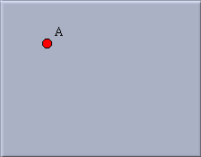Fig. 1: Your first point

Before you add a second point continue reading. If you hold the left mouse button down while adding a point then you can still move it around. The definition of the point will be adapted to the geometric situation at the current location of the mouse pointer (so far there is not a lot of geometry in our drawing but this will change soon). Move the mouse over the drawing surface, press the left button and hold it. Now move the mouse. You will notice that the new point sticks to the mouse pointer. Coordinates that tell the current position are shown. When you approach an already existing point (try it) the new point snaps to the old point. Only after you release the button the new point is added to the construction. If you release the mouse over an old point, no new point is added. Play with these features and add a few new points.

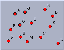Fig. 2: Many points

Undoing an Operation

Your screen may look a bit crowded now. There is an undo-operation that inverts the actions you have performed. By pressing the undo button the last point you added will disappear. Click the undo button until exactly two points remain on the drawing surface. You can use the undo button whenever you make a mistake. You can undo as many consecutive operations as you want.

Moving a Point

We want to continue with our construction of Pappos' Theorem. Place the two remaining points A and B approximately at the position shown in Figure 3.

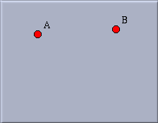Fig. 3: Move to this situation

Most probably your points will not be there. To change this, select the "move" mode by pressing the button in the tool bar. Now, mouse actions in the drawing surface no longer add points; instead, you can pick points and move them around. Move the mouse pointer over the point you want to move. Press the left mouse button. Hold it and drag the mouse. The point follows the mouse pointer. You will also notice that in this mode it does not snap to points. When you release the mouse button the point is placed again. In general, the move mode allows free elements of a construction to be moved. The rest of the construction will change accordingly.

Adding a Line

We are now going to add a line from A to B. Switch to the "Add a line" mode by pressing the button . In this mode you can add a line between two points using a press-drag-release sequence with the mouse. Move over point A. Press the left mouse button. Hold it and move the mouse over point B. Release the mouse.

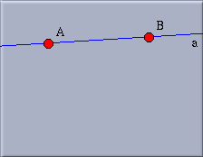Fig. 4: Add a line

This action should have created the desired line. You might have noticed a few things. When you pressed the mouse over point A the point became highlighted. This means that you selected this point as the starting point of the line. While you drag the mouse a second point is always present at the mouse position. When you release the mouse button somewhere this second point will be added. When you approach another point it will be highlighted and the second point snaps to it. You used the second action for attaching the line to B.

If you did not notice these things or made a mistake, undo your operations and try again. Your final picture should look like Figure 4 before you proceed.

Adding More Lines

Now you are ready to add three more lines to end up with Figure 5. You can do this with just three mouse operations. First, move over point B and press-drag to the position of the not yet existing point C. Do another press-drag-release from C to D, and finally from D to E.

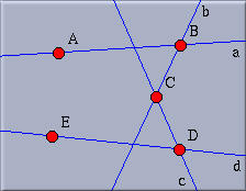Fig. 5: More lines

Observe that you have done all this without leaving the "Add a line" mode. You did some unnecessary work when you added the points A and B in the "Add a point" mode. You could have done this directly in the "Add a line" mode, since not only will the second point be created if necessary, but also the first one. The lines created so far were automatically labelled with the lower-case letters a to d.

Creating Points of Intersection

We stay in the "Add a line" mode. Now we want to draw a line from point E to the intersection of the lines a and c. Move the mouse over E. Press the button. Hold it and move to the intersection of a and c. Release the mouse.

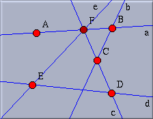Fig. 6: Adding an intersection

When you approached the intersection of the lines they were highlighted and the endpoint of the new line snapped to the intersection. When you released the mouse the new point was defined to be the intersection of the lines. When you will move points A to E the new line will follow the moves accordingly.

The new point F is drawn slightly darker. This means that it is not possible to move F freely in the move mode. F is a "dependent" point. The other points in a construction are "free."

Two things are worth mentioning: With the same procedure you could also have added a "half-free" point that is bound to lie on one line, you just had to release the mouse when you were over one line. All these operations of creating intersections, free or half-free points work similarly in the "Add a point" mode. Many other modes, the interactive modes, also come with this feature. Browse the reference part of this manual for further information.

Finishing the Drawing

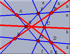
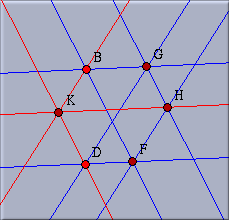
Now it should be easy for you to finish the drawing by adding four more lines. The desired final configuration is shown in Figure 7. First add a line from A to the intersection of b and d. Then draw two lines from A to D and from B to E. Finally, draw a line from C to the intersection of e and f.

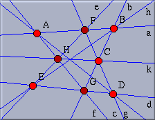Fig. 7: Pappos' Theorem

Now you have added eight points and nine lines. If you look at the configuration you will notice that, if everything was done correctly, the lines g, h and k meet in a point. That this will always be the case in such a construction is Pappos' Theorem. Switch to the move mode by clicking in the tool bar, and drag around the free points of the construction to convince yourself of the truth of this theorem. This theorem was already known to the old Greek geometers. Later it turned out to be of fundamental importance for the theory of Projective Geometry.

Selecting and Changing the Appearance

You may not like the appearance of the drawing. The lines may be too thin and perhaps you want to emphasize the final conclusion of the theorem. Choose the menu item "Properties/Edit Appearance". The following window will pop up:

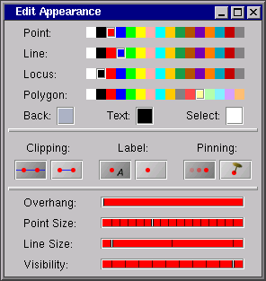Fig. 8: The Appearance Editor

Changes in the Appearance Editor are immediately applied to selected elements. First press the button "Select all lines". If you now move the slider "Line Size" in the Appearance Editor to its second tick, all lines become thicker. After this, switch to "Select" mode . Now, when you click over one or more elements these elements will be selected. If you hold the shift key while you click, the selection state of the element will be toggled.

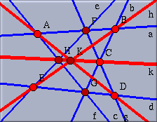
Click over line k, then hold the shift key and click over lines h and g. The lines g, h and k should be highlighted. Click the red box in the second row of the Appearance Editor's color palette. The color of the three lines changes from blue to red. You can also change the size of these lines by moving the "Line Size" slider to its third tick. Finally deselect everything by clicking the button .

Fig. 9: Changed appearance

Adding a Final Point and Proving a Theorem

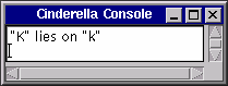
Before you continue open Cinderella's Information Window by choosing the menu item "Views/Information Window". A console window pops up. Cinderella uses this console to report non-trivial facts about a configuration.

We will now create a final point at the intersection of the three red lines. It is hard to use the "Add a point" mode there, since Cinderella refuses to put a point at the intersection of three lines, because the situation is ambiguous. However, you can add a point if you change to the "Meet" mode . This mode expects you to mark two lines. A new point will be added at the intersection of these two lines. Click two of the red lines, say g and h. The new point will be added.

Fig. 10: The point of intersection

Notice that the newly added point K is always incident to line k due to Pappos' theorem. The console reports this remarkable fact automatically.

Fig. 11: A proven theorem

You may wonder how this "proving" works. Cinderella does not use symbolic methods to create a formal proof, but a technique called "Randomized Theorem Checking." First the conjecture "It seems that line k always passes through point K" is generated. Then the configuration is moved into many different positions and for each of these it is checked whether the conjecture still holds. It may sound ridiculous, but generating enough (!) random (!) examples where the theorem holds is at least as convincing as a computer-generated symbolic proof. Cinderella uses this method over and over to keep its own data structures clean and consistent.

Moving Points to Infinity

Let us explore the symmetry properties of Pappos' Theorem. For a nicer picture we want to get rid of the line labels and make the points and lines a bit smaller. First select all lines using . Turn off the labelling by pressing the corresponding button in the Appearance Editor. Change the line size to "thin" (use the slider). Then select all points using . Make them smaller by using the "Point size" slider. Now choose the menu option "Views/Spherical view". What you get will not look very instructive at first sight.

Fig. 12: A spherical view

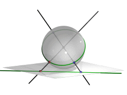
It is a central projection of the plane to the surface of a ball. The projection point is the center of the sphere (see Figure 13). Every point is mapped to an antipodal pair of points, and each line is mapped to a great-circle (an equator) of the ball.

Fig. 13: Projection from the plane to the ball

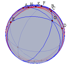
In the spherical view there is a little red slider for controlling the distance of the ball to the original plane. Moving this slider corresponds to a kind of "zooming" operation on the sphere. Please move the slider from its original position much more to the right. Then the situation on the ball should become clearer. If you have adjusted the slider correctly, it should somehow look like Figure 14. You will clearly recognize the construction now drawn on the surface of this ball.

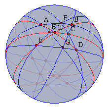Fig. 14: Pappos' Theorem on a ball

The picture needs some explanation: For each point in the plane consider the line spanned by the point and the center of the ball. The intersection of this line with the surface of the ball gives the pair of antipodal points. For each line consider the plane spanned by the line and the center of the ball. The intersection of this plane and the surface of the ball is the great circle that represents the line in the spherical view.

On the sphere there are points that have no correspondence in the Euclidean plane. If the ball touches the Euclidean plane at the "south pole," then the equator of the ball corresponds to the "points at infinity" in the usual Euclidean plane. In Cinderella it is possible to make manipulations in any currently open view. Therefore you can move points also in the spherical view. The changes will be instantly reported to the Euclidean view. In particular, you can grab a point in the spherical view and move it to infinity.

We will do that now, in order to observe that our configuration has a nice three-fold symmetry. Pick point A (in the spherical view) and move it to the 11 o'clock position of the boundary. This point is now really located "at infinity." Notice that in the Euclidean view the lines passing through A became parallel: "The parallels meet at infinity". In a similar way, move point E to the 7 o'clock position and move point C to the 3 o'clock position. Your spherical picture should then look like the ball in Figure 13. In the Euclidean view you find three bundles of parallel lines. You see a kind of Euclidean specialization of Pappos' Theorem. If you like you can try to figure out the corresponding statement in terms of parallels and incidences.

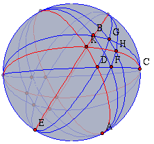Fig. 15: A three fold symmetry

It may happen that the drawing in the Euclidean view is too big or too small. You can use the zooming tools to change this. There is a "Zoom-in" and a "Zoom-out" tool below the Euclidean view. With a press-drag-release sequence you mark the region to (from) which should be zoomed in (resp. out).